
Hyperspectral
While older versions of multispectral sensors could collect data in a few broadly defined spectral bands, during the 1980s, scientists develop an instrument that could measure unprecedented levels of spectral resolution. The hyperspectral instrument was able to collect about 200 sharply defined spectral bands. This new invention was the emerging point of hyperspectral remote sensing [1]. Although there is no clear-cut definition to separate hyperspectral and multispectral imaging, they vary mainly in spectral resolution and bandwidth. Rees et al., for example, defined hyperspectral sensors as devices that can record at least 50 contiguous wavebands [2]. Usually, multispectral sensors measure a limited number of bands (less than 15 bands) with bandwidths ~10-20 nm, while hyperspectral sensors measure hundreds or even thousands of bands in the visible-NIR region (usually from 200-2500 nm) with bandwidth ~0.1-10 nm.
Hyperspectral sensors have different working principles than RGB and multispectral cameras. There are four general hyperspectral imagery techniques, including point scanning (whiskbroom), line scanning (push broom), area (or plane) scanning, and the single-shot (snapshot) method [3]. In the point scanning method, a sensor with a small FOV (~ 4°- 10° ) records reflectance of a target point (or a small area) in broad range (usually 350 nm – 1000 or 2500 nm ) with a relatively narrow bandwidth (can reach below 0.5 nm) delivering a string of reflectance numbers. . On the other hand, the line scanning method uses one slit to measure spectral data on a very narrow line. To capture a hyperspectral image using line scanning, either the sensor or the object should move perpendicular to the scan line. All detector arrays in the scan line usually trigger at once, then the sensor moves forward, and the next line is scanned. Spatial resolution in line scan is determined by the number of detectors in the line array (referred to as cross-track resolution) and forward speed (known as along-track resolution). Although the combination of line scanning sensors with UAVs is not always straightforward, line scanning is the most common scanning method in agricultural remote sensing, mainly because it can deliver high spatial resolution (2 cm or less) depending on the altitude. The third type of hyperspectral sensing is area scanning in which an area is captured once for each single band. This method is similar to RGB and multispectral cameras (they both capture an area) but with much more bands for hyperspectral cameras. As a result, the sensor and object must stay still until measurement in all bands is completed. These types of sensors are rarely used in agricultural remote sensing. Finally, the single-shot method, which is the latest generation of the hyperspectral imaging technique, delivers a data cube including reflectance from a specific area in separate wavelengths all at once. This type of hyperspectral sensors is still in the development stage and mainly used in chemistry and molecular analysis [4].
Hyperspectral cameras are more expensive and complicated than multispectral and RGB cameras that limit their regular applications. However, they provide detailed information about each band's reflectance in a wide spectral range that can be used to pinpoint the most informative bands for a specific phenomenon[5]. For instance, the Chlorophyll Absorption Ratio Index (CARI), which is a strong chlorophyll indicator in plants, uses three relatively narrow bands in the green and red regions[6]. Without using a hyperspectral sensor and finding the relative bands, defining the CARI was difficult. However, once discovered, an inexpensive camera can be devised to captures the informative bands only. Moreover, most external or internal factors somehow affect plants' reflectance that are not entirely identified yet. As a result, many standard reflectance libraries for various materials, including plant leaves, are collected, and being used as a benchmark to answer the different phenomenon's effects on spectral response. For instance, different water treatments might have a footprint on a leaves’ reflectance in specific bands. Comparing the reflectance of the leaves under various water treatments with the standard graph might reveal useful spectral features. Figure 4 shows the standard leaf reflectance of a healthy walnut leaf from USGS library[7]. Since water forms a significant portion of leaves (more than 90% in most healthy leaves), the water absorption bands are noticeable in reflectance graphs. In the reflectance graph both the shape and magnitude should be considered.
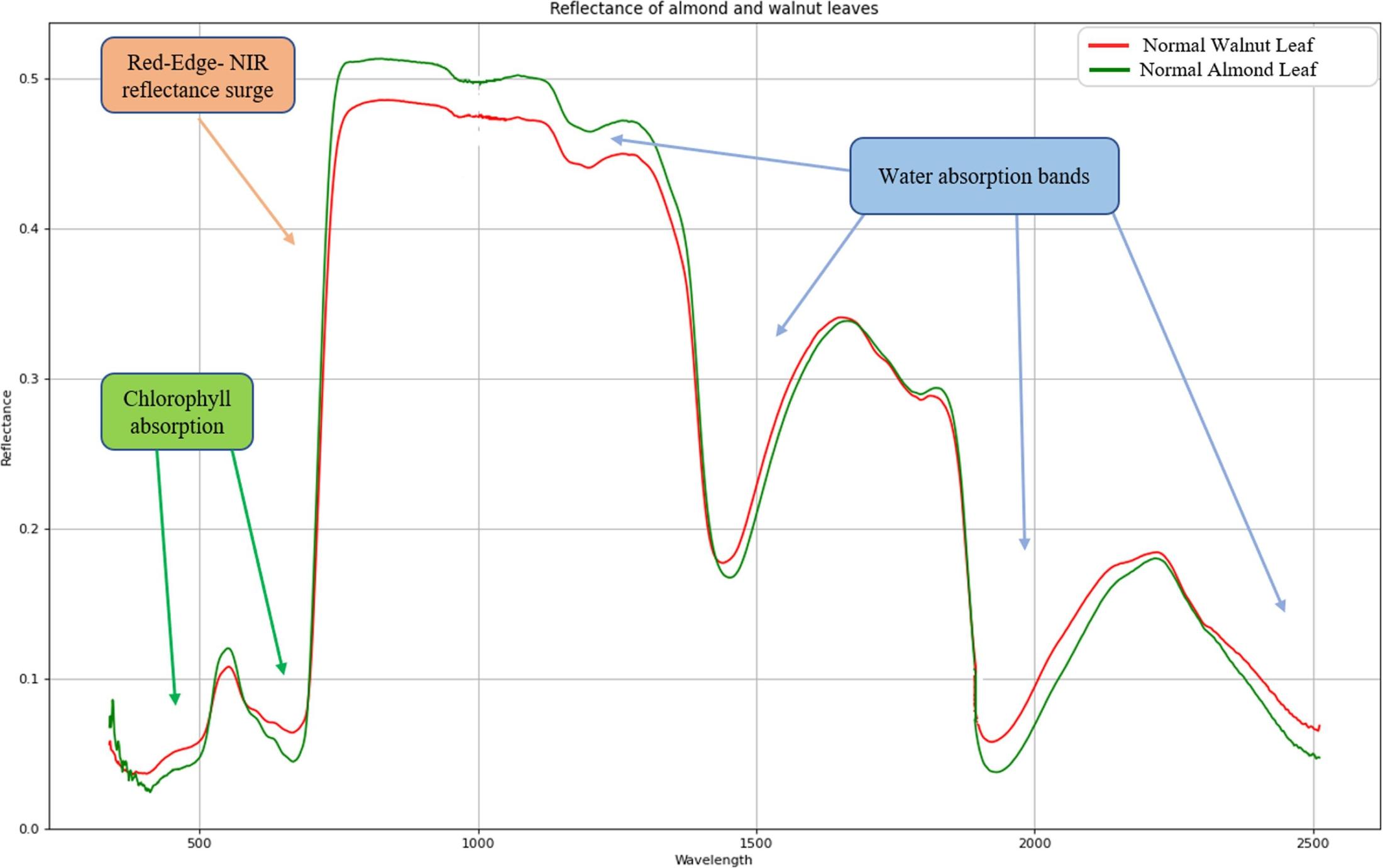
Figure 4- The standard leaf reflectance a walnut healthy leaf from USGS library marked with notable features.
References
[1] J. B. Campbell and R. H. Wynne, Introduction to remote sensing. Guilford Press, 2011.
[2] W. G. Rees, Physical principles of remote sensing. Cambridge University Press, 2013.
[3] D.-W. Sun, Hyperspectral imaging for food quality analysis and control. Elsevier, 2010.
[4] A. Bohlin and C. J. Kliewer, “Single-shot hyperspectral coherent Raman planar imaging in the range 0–4200 cm− 1,” Applied Physics Letters, vol. 105, no. 16, p. 161111, 2014.
[5] R. Omidi, A. Moghimi, A. Pourreza, M. El-Hadedy, and A. S. Eddin, “Ensemble Hyperspectral Band Selection for Detecting Nitrogen Status in Grape Leaves,” arXiv preprint arXiv:2010.04225, 2020.
[6] M. S. Kim, C. S. T. Daughtry, E. W. Chappelle, J. E. McMurtrey, and C. L. Walthall, “The use of high spectral resolution bands for estimating absorbed photosynthetically active radiation (A par),” 1994.
[7] R. F. Kokaly et al., “USGS Spectral Library Version 7,” U.S. Geological Survey, Reston, VA, USGS Numbered Series 1035, 2017. doi: 10.3133/ds1035.